

With financial markets grappling with the disruption of commerce due to the coronavirus, high yield corporate bonds have sold off dramatically. Option-adjusted spreads for US high yield are above 700 basis points (bps), a stress event threshold only breached four other times in the last two decades. While in each of the prior stress events, spreads have widened further, the total drawdown and the duration have not been consistent.
With this in mind, we examine four core considerations for an investor looking at high yield at these elevated spreads: (1) current valuations versus history, (2) the range of return outcomes in prior stress events, (3) the path investors had to experience in reaching those outcomes, and (4) the impact of implementation timeliness on returns.
Current valuations look attractive
Currently over 700 bps, US high yield spreads are in the 86th percentile since 2000 (see figure 1). While the sell-off has so far hit the energy sector the hardest (see figure 2), the general disruption of economic activity has put pressure on high yield spreads more broadly and overall sources of spread are relatively diverse (see figure 3).
What is equally noteworthy to the level of spreads is how quickly valuations changed. US high yield entered 2020 with a little over 330 bps of spread, only about 30 bps above the tightest levels post-Global Financial Crisis, and spreads were under 350 bps in mid-February. The over 600 bps of spread widening observed over the subsequent 30 days was the sharpest month-over-month spread change in index history.
Despite a strong relief rally on the back of Federal Reserve measures, for the year to April 30, 2020, US high yield is still down by a painful 9 per cent. Given the uncertainty surrounding the path of COVID-19 and the economic damage from shutting down large segments of the economy, it is quite possible that spreads will widen again. The goal of this analysis is not to time the bottom of the market, but rather to look to the past for guidance on how spreads have behaved after breaking the 700 bps mark.
Figure 1 – Range of spreads since January 1, 2000
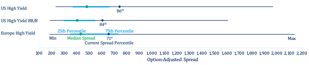
Bloomberg Barclays Indices. Data to April 30, 2020 (which is the “current” date of high yield spreads).
Figure 2 – Spreads (bps) by sector
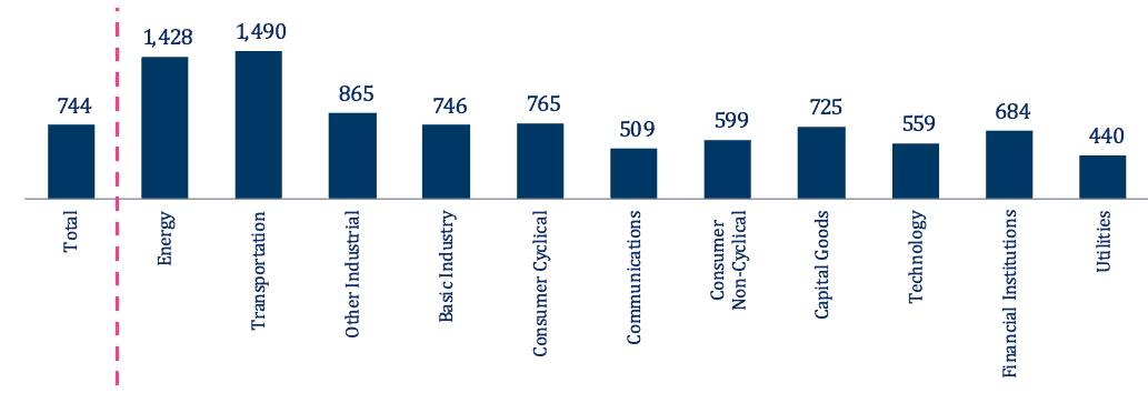
Source: Bloomberg Barclays US High Yield Index, as of April 30, 2020.
Figure 3 – Sources of index spread
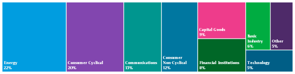
Source: Bloomberg Barclays US High Yield Index, as of April 30, 2020. “Other” includes transportation, utilities and other industrials.
Prior paths through the fog
Since 2000, US high yield spreads have broken through the 700 bps barrier four other times:
- Dot com bubble in 2000
- Global financial crisis in 2008
- European financial crisis in 2011
- Oil price war in 2016
While each incident has its unique characteristics, it can be instructive to look at how high yield debt performed from the outset of stress. This is in many ways the most conservative way to assess returns, as we assume investment exposure throughout the crisis.
Figure 4 – Chart of cumulative high yield returns after hitting 700 bps of spread
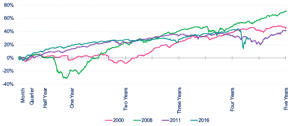
Source: Bloomberg Barclays US High Yield Index. Data to April 30, 2020.
Figure 5 – Table of cumulative high yield returns after hitting 700 bps of spread
| Date | Quarter 1 | Half year |
Year 1 |
Year 2 |
Year 3 |
Year 4 |
Year 5 |
Maximum drawdown |
| October 19, 2000 | +1% | +1% | -3% | -8% | +24% | +39% | +46% | -8% |
| January 22, 2008 | +3% | +1% | -20% | +23% | +41% | +48% | +71% | -31% |
| August 9, 2011 | +3% | +7% | +14% | +24% | +34% | +33% | +42% | -5% |
| January 12, 2016 | +5% | +13% | +19% | +28% | +28% | +43% | -4% |
Source: Bloomberg Barclays US High Yield Index with calculations by Mercer.
Notes: figure 5 is for informational and illustrative purposes only. Cumulative total return is calculated using the percentage change in the index value, which includes reinvestment, from the start date to the end date. The start date is determined by when the index first pasts the 700 bps OAS threshold used to determine a stress event. The end date is a fixed length of time from the start date as described in the table. Time periods have been selected with the benefit of hindsight based on actual historical data and not based on assumptions. Past performance is no guarantee of future results. It is not possible to invest directly in an index. Index returns are gross of fees, transaction costs, or other expenses and include reinvestment of coupon income.
In all periods shown, cumulative absolute returns were meaningfully positive by the third year, despite the losses associated with defaults and the potential impact of fallen angels. However, what is important to mention is the volatility that comes with investing early in a credit cycle downturn. In all cases, there were more losses yet to come, with the maximum total losses another 4 to 31 per cent away. To reap the reward of the elevated level of spreads, investors will have be prepared to endure meaningful volatility and drawdowns.
Being realistic about implementation
Even if one is convinced that high yield will win out over the long run, the question remains of how timely an investor needs to be. With competing investment priorities, governance processes, and the general fear of the unknown, it can be easy to delay on a given investment. Whilst past performance is no guide to the future, we show in figure 6 how the cumulative returns of the initial three-year time period would have been impacted by a variety of delays to the investment.
Figure 6 – Impact of delayed investment on cumulative three-year returns (relative to no delay)
| Date/Delaying by | One month |
One quarter |
Two quarters |
Three quarters |
One year |
| October 19, 2000 | +2% | -1% | -1% | -1% | +3% |
| January 22, 2008 | 0% | -5% | -1% | +37% | +35% |
| August 09, 2011 | -1% | -4% | -9% | -13% | -16% |
| January 12, 2016 | +6% | -6% | -14% | -18% | -21% |
Source: Bloomberg Barclays US High Yield Index with calculations by Mercer.
Notes: figure 6 is for informational and illustrative purposes only. Cumulative total return is calculated in a similar manner to figure 5, except rather than fixing the start date, the end date is fixed at three years from when the index first passes the 700 bps OAS threshold used to determine a stress event. The start date is modified by the amount specified in the table from the date when the index first passes the 700 bps OAS threshold. Time periods have been selected with the benefit of hindsight based on actual historical data and not based on assumptions. Past performance is no guarantee of future results. It is not possible to invest directly in an index. Index returns are gross-of-fees, transaction costs, or other expenses and include reinvestment of coupon income.
The impact of delaying investment has been mixed, which is not surprising since we start the clock near the beginning of a credit downturn. In the two most recent cases, delaying the investment by more than one quarter had a meaningful impact on results, as the initial snap back in spreads was missed. However, in the global financial crisis, the depths of the crisis were not reached until around a year after spreads reached 700 bps.
History is only a guide not a guarantee
While staring into the unknown can be daunting for any investor, the past may provide perspective on future outlook. What this piece has aimed to provide, historical perspective, is only a single puzzle piece in constructing an investment thesis for high yield at elevated spread levels. Investors will still need to consider the unique circumstances of the current sell-off as well as the suitability for their own portfolio needs and risk tolerance.
Nathan Struemph is a fixed income asset class specialist at Mercer.


Leave a Comment
You must be logged in to post a comment.
Login