

How can portfolio construction handle the challenge of ‘good and bad’ scenarios?
Uncertainty is ever-present whether related to health, social, economic, market, geopolitical or a myriad of other areas. There are many possible scenarios which form in our minds and the challenge is to incorporate these insights into our portfolio construction decisions. The question is how to best integrate scenarios into portfolio construction.
Academics have been actively exploring these types of problems for decades – indeed it has been a research interest for some of the most well-known and respected names in financial academia. In this article I look at some of these techniques and their usefulness for investors, but first we need some background. Some of the academic approaches have great merit but are difficult to apply in practice.
A primer on portfolio construction
Basic portfolio construction theory, as applied by industry, is built on three inputs: estimates of expected return and variability (typically volatility) to summarise the distribution of asset returns, accompanied by a clear objective. Given the prevalence of labelled products (e.g. balanced, growth etc.) and peer group awareness in industry, the objective is commonly to maximise return for a fixed level of risk. This is broadly reflected in what is classically known as the mean-variance framework.
Commonly this standard approach is complemented by stress tests and scenario analysis to explore the impact of extreme events.
How do we account for uncertainty and possible scenarios?
Return to the outlined problem: investors are uncertain of the future and identify many possible scenarios. Can these scenarios be accounted for in portfolio construction? To keep the analysis as simple as possible consider only one risky asset (stocks) and define two scenarios (good and bad). Then consider the more detailed problem (a “real world” setting) of multiple asset classes which helps to illustrate the complexity-based barriers to industry adoption.
Simplified case of stocks only
I assume a one-year timeframe because it most conveniently illustrates the outcomes of different techniques. Our two scenarios are defined as follows:
- A good scenario (70% likely) where expected real stock returns are 20%
- A bad scenario (30% chance) where expected real stock returns are -10%
For both scenarios stock volatility is assumed to be 12%.
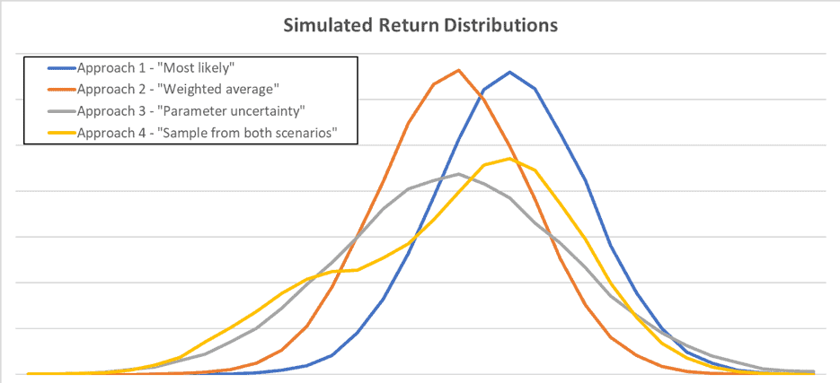
The first approach uses the most likely scenario, in this case the good scenario where expected real stock returns are 20%. The problem with this approach is obvious: by not incorporating our knowledge of the alternative scenario it fails to consider the full range of possible market outcomes. As can be seen in the diagram and table below (blue line) the expected return is overstated and volatility is understated (compared to the more advanced techniques). This would result in a flawed decision to over-allocate to stocks.
A second approach calculates expected return as a probability-weighted average of these two scenarios (so expected stock returns are 11% real). As displayed by the orange line in the diagram, the bias in expected returns identified in the first approach is removed, but the range of potential outcomes remains understated as this approach ignores the existence of two distinct scenarios. This approach would still result in over-allocating to stocks.
A third approach applies a technique known as parameter uncertainty. This approach also uses the weighted average expected return, but acknowledges that there is uncertainty around the expected return itself (after all it is unknown which scenario will be experienced). The expected real return is 11% real but, based on two possible scenarios, the expected return itself has a standard deviation of 12%[i]. So, in simulating possible outcomes the expected return itself is simulated and then the return itself. The return distribution (illustrated by the grey line) is much wider (simulated volatility is over 18%) which would reduce the optimal demand for stocks. However, this approach still doesn’t perfectly translate our two-scenario view into portfolio construction.
The final approach does just that. It samples from the two scenarios to form a distribution of possible outcomes from investing in stocks. The volatility remains high but the diagram (yellow line) shows the presence of two scenarios in the return distribution itself. This approach best incorporates knowledge of possible scenarios.
| Simulation results | Approach 1 – “Most likely” | Approach 2 – “Weighted average” | Approach 3 – “Parameter uncertainty” | Approach 4 – “Sample from both scenarios” |
| Average | 20.1% | 11.1% | 10.3% | 11.9% |
| Standard Deviation | 12.1% | 12.1% | 18.4% | 18.6% |
In practice it is complex
It appears logical for portfolio construction approaches to account for possible scenarios. I’ve illustrated the benefits using the simple case of stocks. But this is the crux of the issue: it is a simplified setting. Let’s consider a more detailed problem.
To apply the scenario sampling approach in a broader setting requires the need for parameter estimates (expected return) for every candidate asset under each scenario. There is an important reflection here: unless all the individual asset return forecasts move in perfect unison across each scenario, there will be a different optimal portfolio for each scenario. So, what is the optimal portfolio across all scenarios? This is a complex problem which requires a lot of computational power to solve, which becomes even more complex as more scenarios are considered.
Hopefully it is now easier to understand why the theoretically appealing portfolio construction practices used by academics aren’t commonly replicated in industry. However, there are two important learnings that can be taken from academia. First, forecasts are only point estimates and are uncertain so it would make sense to acknowledge this forecasting uncertainty when constructing portfolios. The second learning is that scenario analysis, already part of good industry practice, could be extended to consider not only extreme scenarios, but likely scenarios as well.
[i] This is estimated based on a Bernoulli distribution.
David Bell is executive director of The Conexus Institute.


Leave a Comment
You must be logged in to post a comment.
Login