

Defensive equity investment strategies are nothing new, but a key issue with many is that defensive does not necessarily mean low volatility. Scientific Beta looks at a strategy to target both goals, using robust low volatility controls to create a new defensive index for the volatility-averse investor.
Traditional defensive strategies have been popular for many decades. In addition to providing relative protection in bear markets, they benefit from the positive long-term premia associated with the low volatility factor.
Unfortunately, we can observe that the popular low volatility strategies’ strong tilt towards value is often associated with negative exposures to the other rewarded factors, which deprives these strategies of the potential for long-term risk-adjusted performance.
To respond to this shortcoming, it is possible to apply a high factor intensity filter to a defensive strategy, which removes the highly negative exposures to other rewarded factors.
This type of approach harvests the low volatility factor while maintaining positive exposures to other rewarded risk factors.
Figure 1: Low Volatility Strategies’ Exposures to Rewarded Risk Factors
| 21-Jun-2002 to 31-Dec-2019 (RI/USD) | SciBeta Developed HFI Low Volatility DMS (4-Strategy) | SciBeta Developed Narrow HFI Low Volatility DMS (4-Strategy) | MSCI World Minimum Volatility |
| Sharpe Ratio | 0.85 | 0.86 | 0.70 |
| Size (SMB) Factor | 0.10 | 0.08 | 0.10 |
| Value (HML) Factor | 0.09 | 0.08 | -0.12 |
| Momentum (MOM) Factor | 0.05 | 0.04 | -0.04 |
| Low Volatility Factor | 0.32 | 0.43 | 0.42 |
| Profitability Factor | 0.09 | 0.01 | -0.04 |
| Investment Factor | 0.03 | -0.02 | -0.04 |
| Factor Intensity (Int) | 0.68 | 0.62 | 0.27 |
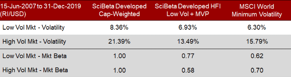
However, traditional defensive strategies are not always low volatility and unfortunately, in absolute terms, can exhibit strong peaks in volatility, notably in periods of crisis, like highly volatile market conditions, when the investor would like to be genuinely protected.
One solution is to combine a traditional defensive strategy with a tool that minimises volatility to create an index that offers both benefits. For example, a maximum volatility protection risk control strategy, or MVP, is fairly easy to implement, smooths volatility through time and reduces its peaks.
To smooth volatility, it is of course necessary to forecast it. That is why a volatility forecasting model, which takes into account properties such as volatility clustering, leverage effect or fat-tailness, is necessary. Using this good volatility forecast, it is then easy, in an expected period of strong volatility, to reduce market exposures, which are the main source of the portfolio’s volatility, using a futures overlay. MVP delivers low volatility in all market conditions, especially when investors need it most. Reduced market exposure in periods of high volatility shrinks downside risks and allows Sharpe ratios to be improved, improving risk-adjusted performance over the long-term. Given its innovative nature, we provide details below on the benefits of the MVP strategy and how it works.
Maximum Volatility Protection: a new way of smoothing out returns
The MVP’s objective is to cap volatility at the historical volatility of the underlying defensive index with which you combine it. This can achieved by a monthly allocation to a CW overlay, determined by two elements:
- The volatility target, which is set as the historical volatility of the selected defensive index;
- The volatility forecast over the next month. The forecast is based on a robust model that captures the main stylised facts of financial returns. Since the objective of the MVP risk control option is to cap the volatility of the new defensive solution at the volatility target, the allocation (WOverlay) to the CW Overlay is set as follows:
![]()
where σtarget is the volatility target, σforecast is the volatility forecast over the next month and is the market beta of the defensive index.
The allocation to the CW overlay can only be negative, ie when the volatility forecast is below the target we have a zero allocation to the CW overlay and the new defensive solution is fully exposed to the underlying index.
When the volatility forecast is above the target, then we take a short position in the CW overlay (as defined above), which allows market exposure to be reduced. The CW overlay can be replicated using futures, which makes it very simple to implement. Indeed, futures are very liquid instruments with no counterparty risks and they are cheap to trade. Moreover, the allocation to the index is always 100 per cent, so almost no additional turnover is linked to this implementation.
However, certain institutional investors face governance or regulatory constraints that hinder them from using a CW overlay.
For them, we suggest a physical implementation that requires a dynamic allocation between the underlying index and cash. Like the CW overlay implementation, we impose a no-borrowing constraint on cash that implies the allocation to the index is limited to maximum of 100 per cent.
Of course, this implementation can generate significant additional turnover because of round trip allocations that might be non-optimal.
Therefore, to improve the replicability of the physical implementation, we can apply turnover control to limit the turnover while conserving the effectiveness of the MVP approach. The main challenge in implementing the MVP is to accurately forecast the volatility. Our forecasting model is an asymmetric GARCH4 model to forecast volatility with student-t innovations. This model captures financial returns stylised facts such as volatility clustering, leverage effect and fat tails. We tackle structural breaks by using two forecasts based on an expanding window and a five-year rolling window.
The key benefits of using Maximum Volatility Protection risk control
Figure 2 compares the MVP’s one-year rolling volatility compared to that of traditional defensive indices, it’s clear that it provides much more stable volatility and significant reduction of volatility peaks during market distressed regimes, such as the financial crisis of 2008 or the European crisis of 2011.
Figure 2: Maximum Volatility Protection to Avoid Volatility Peaks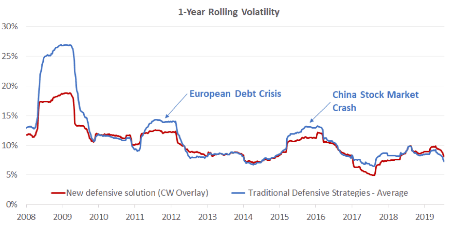
We use three different traditional defensive strategies to get an average 1-Year rolling volatility: MSCI World Minimum Volatility,
FTSE Developed Minimum Variance and Robeco QI Institutional Global Developed Conservative Equities. Sources: Scientific Beta, DataStream and Bloomberg
It achieves this volatility smoothing thanks to a dynamic allocation to either the CW overlay or the underlying defensive index. For example, during the 2008 financial crisis and 2011 European debt crisis, the allocation to the index was massively reduced. During the 2008 financial crisis, the reduction was more than 70 per cent for the physical implementation and 54 per cent for the CW overlay implementation.
There are also two very recent events that generated strong reduction of exposure to the underlying defensive index.
- First, on February 5, 2018, the Dow Jones had its worst point decline in history when the index closed with a negative performance of -4.6 per cent. This event generated a strong exposure reduction to the underlying index at the February rebalancing.
- Second, the final quarter of 2018 was marked by a poor equity market performance following fears of an imminent economic downturn after the most important bull market in recent history. Our volatility forecast model reacted very quickly and exposure to the underlying index was reduced significantly in October and December.
Finally, we underline the differences in the variations of allocations through months between both implementations. The CW overlay implementation has no turnover control and reacts therefore more quickly to change in volatility forecasts from month to month than the physical implementation.
The MVP risk control strategy has a very interesting impact on the conditional market beta and volatility measures. Both are strongly reduced in high volatility market regimes and almost identical to the underlying index in low volatility regimes. This dissymmetry is at the heart of the success of the MVP risk control strategy.
Figure 3: Reduction of Market Beta and Volatility in Distressed Times
A modern solution to volatility protection
The defensive strategy that we have summarised is unique in the indexing industry. It is nonetheless easy to implement if one has a good capacity to forecast volatility. This new solution allows volatility to be smoothed through time and consequently improves average and extreme risks as well as the Sharpe ratio. Investors worried about a possible market downturn after the longest bull market observed over the recent history should consider this new defensive strategy.
Daniel Aguet is head of indices at Scientific Beta, Noël Amenc is chief executive at Scientific Beta and Associate Dean for business development at EDHEC Business School, and Felix Goltz is research director at Scientific Beta.


Leave a Comment
You must be logged in to post a comment.
Login